How To Create Pivot Table In Microsoft Excel To Analyze Excel Data In Excel Sheets and Google Sheets

 Pivot Table in Google Sheets and Excel Sheets

Pivot Tables are most used and powerful feature of Microsoft Excels to calculate, analyze and summarize data in quick and handy manner. That enable you to get summarized data. It is quite useful tool that is being used in organizations.

Let's learn how to perform and create pivot table in both Excel and Google sheets.

Table of content:

1. How To Create Pivot Tabel In MS Excel Sheets - Step by Step

1.2 What are the features of using Pivot Table

2. Create Pivot Tabel In Google Sheets - Step by Step Guide

(1) How To Create Pivot Tabel In MS Excel Sheets - Step by Step:

Step 1: Here is the data for which I have to create Pivot Table:

Step 2: Go to Insert Menu and Click Pivot Tabel; as the screen as below:

• Excel by default selects the table range, you can also change or select wherever your data exists.

• Default Pivot Table's address is New Worksheet you can change through the Existing Worksheet Option.

Step 3: Press Ok and You will get directed to the Pivot Table as;

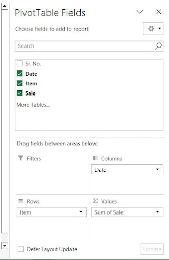
Step 4: Next add the pivot table field values as shown in below image;

Step 4: And, your Pivot Table summarize data looks like this;

Pivot Tables are very useful in Microsoft Excel powerful quick method.

You don't need create every time it; it there is a change or update in your data;

You just need to go Pivot Table, Right click and Just Refresh it :-

What are the features of using Pivot Table?

• To get summarize data 
• Quick and Easy summary of large database
• Get an accurate data in a minute

(2) Create Pivot Tabel In Google Sheets - Step by Step Guide:

Step 1: Get your data ready first for which you have to create a Pivot Table

Here is an example of it as below image:

Step 2: Go to Insert Menu and Click Pivot Tabel and You will get the the screen as below:

3. Enter Create(Excel automatically selects the data range hence it can changed).

And, Excel's default Pivot Table location is New Sheet(change if you want)

4. Your new sheet of Pivot Table looks like below;

4. Next, Adjust the data field;

4. As the above image shows I have added Item column in columns section and in the values section I put Sale column.

Here is the summarize data on above selection:

This is how Pivot Table are easy to use within a few minutes.