An Excel Vlookup function tutorial with example — Microsoft Support — Basic Excel Formula
The basic VLOOKUP function for beginners and Advanced Users: An Excel Function ‘VLOOKUP’ is basic excel function used by students and professionals — for commercial and corporate offices use also. The Microsoft Office VLOOKUP function in In Microsoft Excel Sheet and Google Sheet is use to search and get data from a range or table of well organised data.
The VLOOKUP Function Syntax:
VLOOKUP(search_term, range, index(is_sorted])
The Vlookup stands for “Vertical Lookup” function. It returns data for the exact match of search key/value (use it to search for an item in a column and return data from that row if a match is found). The search values should be compulsory exact match with the table data or range of data you are searching for.The VLOOKUP function in Google Sheets is typically used to bring data from one data table and add it into another.
Points to be noted white using Microsoft Excel function —
- The search term must be available or present in the data or table where you have to look for.
- The search term must be the same and exact in the table data. It should not contain any space or other; must be same as in data.
- The data/table of information is required for lookup.
Vlookup function used to find related records: VLOOKUP can also handle approximate matching as well as wildcard searches. These more advanced use cases are explored further below.
How to use excel vlookup function — Microsoft support:
- The name VLOOKUP stands for Vertical Lookup.
- As it name suggests it searches for a value up and down a column meanwhile vertically, rather than horizontally.
- The vlookup function always starts with “=” sign similarly as all the basic excel formulas and function following up by the function name “vlookup”; opening bracket. Then select the cell or enter the search term manually.
- It would be best to use cell reference or cell address.
- Now select the column in which you have to look up for search term. Now select the index number of which column data you want to get as result. The search key is the item from the original table that you want to search for in the lookup table.
- VLOOKUP always searches down the first column of this table. If the search term is found, the value from a specific cell of that row is returned. The index value (the third argument) determines which column of the lookup table to use.
Here are some basic most important things you must know about it:
- It does exact matching.
- It is not case sensitive.
- If there are multiple matches found in the data/table, the first match is found and the returns the value of first reference.
- If no lookup value is found, VLOOKUP returns the #N/A error message.
Let’s get start with some examples :
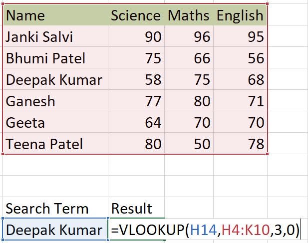
In the following example; there is data of students marks obtained different subjects like Maths, Science and English. Now here I am starting with and looking for the particular student marks in particular subject.
- I have to lookup for Deepak Kumar’s marks obtained in maths as follow:

And, the result of the search is :

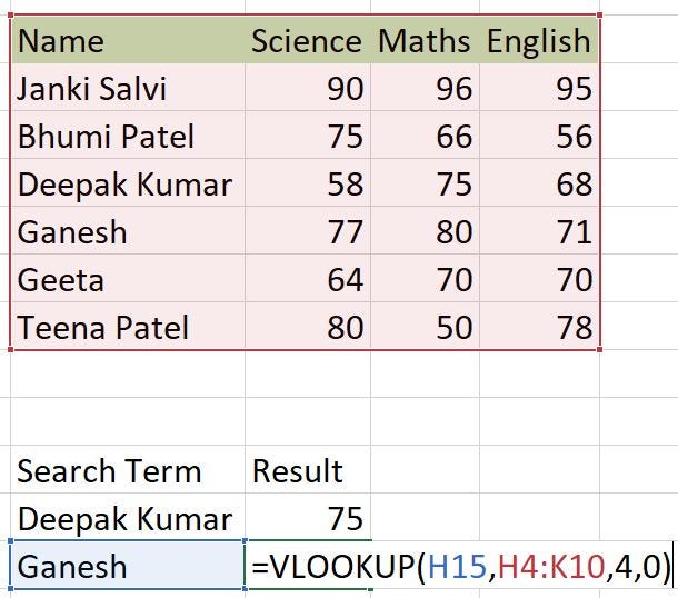
2. Next, in the same table I’m looking for marks of English subject for Ganesh.
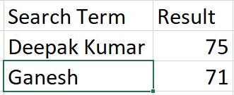
And, the result is as follow:

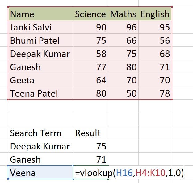
3. Now I’m looking for the marks of science subject obtained by Veena.
Now it returns #NA as the function is unable to found match for “Veena” in the array or in the table.

